The Mass Spring Damper System
The study and analysis of the dynamical behavior of mechanical systems give us many insights into fundamental concepts governing motion (e.g., frequency, damping, and stability). A simple mechanical system that is widely adopted in academia for explaining the before-mentioned concepts is the Mass Spring Damper system. In the following figure, a schematic diagram of the mass-spring-damper is depicted.
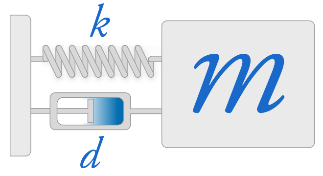
The mass is attached to two components: the spring and the damper, both of which are connected to a fixed frame. The first step to be fulfilled before our analysis is the creation of a mathematical model that encapsulates all the critical dynamical behavior for our system.
In this article, a model for the mass-spring-damper system will be represented, and the implementation of the model will be illustrated. After that, the free response will be studied under certain initial conditions.
1) Description
It is crucial to emphasize the difference between the influence of the spring and the damper on the overall dynamical behavior of the system. As can be seen in the following figure, three sliding switches have been added near the linking points of (i) the spring, (ii) the damper and (iii) the applied force for the purpose of clarification.
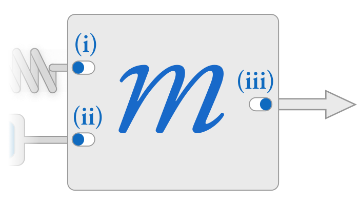
The sliding switches are used to demonstrate whether there is a reaction force at a specific position or state or not, and it also gives information on the direction of the reaction force. As shown below, the three sliding switches are illustrated in the case of three states: the equilibrium state, the moving state, and the still state.
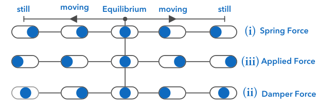
The equilibrium state describes the system when it is at rest with no applied or reaction forces exhibited on the system. By looking at figure 3, one can see that the three switches are positioned in the center, which means that no (i) spring, (ii) damper or (iii) applied force acting on the mass. The second state is the moving state, illustrated in both the left and right directions. Once a force is applied on the mass, the mass begins to change its position at a certain velocity, and thereby both the spring and damper exhibit a reaction force that opposes the movement of the mass. The last state is the still state. The still state explains the situation where an applied force displaces the mass out of its equilibrium state, and the mass is standing still in its new position with zero velocity. In the current state, the spring counteracts the displacement with a reaction force, while the damper doesn't exhibit any reactions since the mass is not moving.
Therefore, the damper reacts only when the mass is moving or has a certain velocity. On the other hand, the spring force is only present when the mass is displaced from its equilibrium position. To put it simply, the damper counteracts the velocity, whereas the spring force opposes displacement. Note that, this deduction is based on a linear damper and a linear spring.
2) Modeling:
The equation of motion of the MSD system is expressed by the following linear ordinary differential equation:
$$ \begin{equation} m\ddot{x} + d\dot{x} + kx = f(t) \end{equation} $$Where the coefficients in the reaction forces are the damper's coefficient $d$ (measured in Kg/s) and the spring's coefficient $k$ (measured in Kg/s2).
There are two other equivalent representations to eq.1. First, the transfer function,
$$ \begin{equation} \frac{X(s)}{F(s)} = \frac{1/m}{s^2 + (d/m)s + (k/m)} \end{equation} $$and, second, the state space representation:
$$ \begin{equation} \begin{bmatrix} \dot{x}_1 \\ \dot{x}_2 \end{bmatrix} = \begin{bmatrix} 0 & 1 \\ -(k/m) & -(d/m) \end{bmatrix} \begin{bmatrix} x_1 \\ x_2 \end{bmatrix} + \begin{bmatrix} 0 \\ 1/m \end{bmatrix} f(t) \end{equation} $$At this point, we have three equivalent representations of the system. The first representation is the second order differential equation (eq.1). The second representation is the transfer function (eq.2), and the last representation is the state space representation (eq.3).
All three equations (eq.1, eq.2 & eq.3) encapsulate the linear dynamical behavior of the mass-spring-damper system, and they are all equivalent.
3) Analysis:
In what follows, we'll investigate the free response of the system. The linear ODE, represented by eq.1, will be used to understand the behavior of motion.
First, we'll transform eq.1 into the standard form by dividing by the mass $m$. After division, the standard form of the Mass Spring Damper system model is written as follows:
$$ \begin{equation} \ddot{x} + 2\zeta\omega_n\dot{x} + \omega_n^2 x = f_m(t) \end{equation} $$The standard form of the equation has two principal coefficients: the damping ratio $\zeta$ and the natural frequency $\omega_n$. The value of the damping ratio will be used to distinguish between different cases of motion. Another coefficient is the mass-normalized applied force $f_m(t)$. Since we're studying the free response, this coefficient is going to be zero. The three coefficients are formulated as follows:
$$ \begin{equation} \zeta = \frac{d}{2\sqrt{km}}, \qquad \omega_n = \sqrt{\frac{k}{m}}, \qquad f_m(t) = \frac{f(t)}{m} \end{equation} $$The homogeneous linear ordinary differential equation of the system is written as follows:
$$ \begin{equation} \ddot{x} + 2\zeta\omega_n\dot{x} + \omega_n^2 x = 0 \end{equation} $$The initial conditions, the initial velocity and the initial position, are defined as follows:
$$ \begin{equation} x(0) = x_o, \qquad \dot{x}(0) = v_o \end{equation} $$Because the damping ratio and the natural frequency in eq.6 are not functions of time, we know that a solution is exponential in nature, or,
$$ \begin{equation} x = e^{\lambda t} \end{equation} $$By finding the first and second derivatives for the last expression:
$$ \begin{equation} \dot{x} = \lambda e^{\lambda t}, \qquad \ddot{x} = \lambda^2 e^{\lambda t} \end{equation} $$And then substituting into eq.6, we get
$$ \begin{equation} \left(\lambda^2 + 2\zeta\omega_n\lambda + \omega_n^2\right)e^{\lambda t} = 0 \end{equation} $$By dividing both sides by the exponential term, we get:
$$ \begin{equation} \lambda^2 + 2\zeta\omega_n\lambda + \omega_n^2 = 0 \end{equation} $$The two solutions of the characteristic equation (eq.11) are
$$ \begin{equation} \lambda_{1,2} = -\zeta\omega_n \pm \omega_n\sqrt{\zeta^2 - 1} \end{equation} $$Based on the sign of the discriminant of eq.12, three different roots will result. First, when the value of $\zeta$ is less than 1 (i.e., $\zeta < 1$), two complex conjugate roots with negative real parts will result. This corresponds to the Underdamped Motion, where the motion is oscillatory and decays as time advances. Second, if the value of $\zeta$ is equal to 1 (i.e., $\zeta = 1$), two negative real roots having the same value will result; this corresponds to the Critically Damped Motion, the case where the motion is non-oscillatory. The third and last case is when the value of $\zeta$ is greater than 1 ($\zeta > 1$). In this case, two real and distinct roots will result. The behavior of motion, in this case, is called Overdamped Motion, where the motion has no oscillations and decays at a slower rate than that of the critically damped motion. In what follows, we will go through each case in succession.
a) Underdamped Motion:
By reforming the two values of $\lambda$, defined in eq.12, to accommodate to the underdamped case, where the damping ratio has a negative value, we get:
$$ \begin{equation} \lambda_{1,2} = -\zeta\omega_n \pm j\omega_n\sqrt{1 - \zeta^2} \end{equation} $$Note that the imaginary part in the last expression is defined as the damped natural frequency, denoted by $\omega_d$:
$$ \begin{equation} \omega_d = \omega_n\sqrt{1 - \zeta^2} \end{equation} $$By substituting the values of these roots in the main exponential function (eq.8), we get the two solutions (i.e. basis of solutions)
$$ \begin{equation} x_1 = e^{\lambda_1 t}, \qquad x_2 = e^{\lambda_2 t} \end{equation} $$To find the general solution, we'll multiply each solution in eq.15 by a constant and add the resulting expressions:
$$ \begin{equation} x = c_1 e^{\lambda_1 t} + c_2 e^{\lambda_2 t} \end{equation} $$By substituting the values of the roots, eq.13, into the general solution, eq.16, we arrive at the position equation $x(t)$ of the free response in the underdamped case:
$$ \begin{equation} \boxed{x = e^{-\zeta\omega_n t}\left(c_1 e^{j\omega_d t} + c_2 e^{-j\omega_d t}\right)} \end{equation} $$The constants $c_1$ and $c_2$ in the last expression are complex, and are defined by:
$$ \begin{equation} c_1 = \frac{x_o\omega_d - j(v_o + x_o\zeta\omega_n)}{2\omega_d}, \qquad c_2 = \frac{x_o\omega_d + j(v_o + x_o\zeta\omega_n)}{2\omega_d} \end{equation} $$We could express the solution defined by eq.17 using Euler's formulas to get rid of the imaginary terms and have a more clear representation, which is:
$$ \begin{equation} \boxed{x = A\,e^{-\zeta\omega_n t}\sin(\omega_d t + \phi)} \end{equation} $$As you can see, the expression, defined by eq.19, represents a decaying sine wave equation with amplitude $A$, frequency $\omega_d$ (in rad/s) and phase shift $\phi$. The exponential term determines the decaying rate of the transient underdamped response. The values of the amplitude and phase shift are:
$$ \begin{equation} A = \frac{\sqrt{(x_o\omega_d)^2 + (v_o + x_o\zeta\omega_n)^2}}{\omega_d}, \qquad \phi = \arctan\left(\frac{x_o\omega_d}{v_o + x_o\zeta\omega_n}\right) \end{equation} $$The position of the mass against time is shown in the following figure, fig. 2.
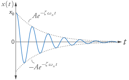
In figure 3, the mass is subjected to an initial position. The curve begins at the initial position $x_o$ and, then, dies out with an oscillatory behavior. The exponential term defines the decaying rate of the sinusoid.
b) Critically Damped Motion:
By reforming the two values of $\lambda$ that correspond to the critically damped case, $\zeta = 1$, we get one value for the roots and not two as before:
$$ \begin{equation} \lambda_{1,2} = -\zeta\omega_n \end{equation} $$The value of the roots is real and negative. Since we have only one value for the roots, we get only one solution from two sufficient solutions to form a general solution. By substituting the value of the roots eq.21 into eq.8, we get a solution from two:
$$ \begin{equation} x_1(t) = e^{-\zeta\omega_n t} \end{equation} $$In order to find the second solution, we'll use the reduction of order method, or simply, in our case, we'll multiply the first solution by the time. The second solution will be:
$$ \begin{equation} x_2(t) = t\,e^{-\zeta\omega_n t} \end{equation} $$By multiplying both the first and second solutions, eq.22 and eq.23, by the constants $c_1$ and $c_2$ then adding the resulting expressions, we get the general solution of the critically damped case:
$$ \begin{equation} \boxed{x(t) = c_1 e^{-\zeta\omega_n t} + c_2\,t\,e^{-\zeta\omega_n t}} \end{equation} $$Using the initial conditions, we'll find the values of the constants:
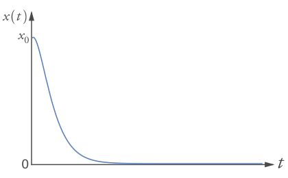
$$ \begin{equation} c_1 = x_o, \qquad c_2 = v_o + x_o\zeta\omega_n \end{equation} $$The free response of the critically damped type doesn't contain any oscillations; the motion smoothly approaches zero as time advances. The behaviour of the critically damped motion is depicted in the following figure.
c) Overdamped Motion:
The two values of $\lambda$ that correspond to the overdamped case, where $\zeta > 1$, are real and distinct. They are written as follows:
$$ \begin{equation} \lambda_{1,2} = -\zeta\omega_n \pm \omega_n\sqrt{\zeta^2 - 1} \end{equation} $$The general solution of the ordinary differential equation is
$$ \begin{equation} x(t) = c_1 e^{\lambda_1 t} + c_2 e^{\lambda_2 t} \end{equation} $$By evaluating the values of the roots, eq.26, into the general solution, eq.27, we get the position equation of the free response in the overdamped case:
$$ \begin{equation} \boxed{x(t) = e^{-\zeta\omega_n t}\left(c_1 e^{\omega_n\sqrt{\zeta^2 - 1}\,t} + c_2 e^{-\omega_n\sqrt{\zeta^2 - 1}\,t}\right)} \end{equation} $$The constants $c_1$ and $c_2$ in the last expression are defined by:
$$ \begin{equation} c_1 = \frac{x_o\omega_n\left(\sqrt{\zeta^2 - 1} + \zeta\right) + v_o}{2\omega_n\sqrt{\zeta^2 - 1}}, \qquad c_2 = \frac{x_o\omega_n\left(\sqrt{\zeta^2 - 1} - \zeta\right) - v_o}{2\omega_n\sqrt{\zeta^2 - 1}} \end{equation} $$It is also interesting to see the position versus time plot that corresponds to the overdamped motion, shown in the following figure.
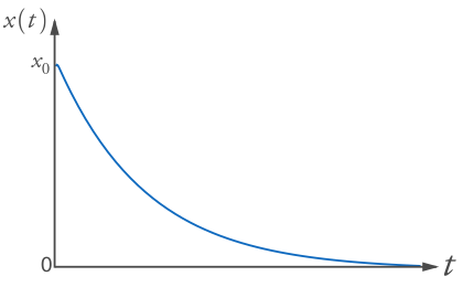
It is clear that the motion exhibits a non-oscillatory behaviour.
An illustration of the three types of motion, the underdamped motion, the critically damped motion and the overdamped motion, is depicted in the figure. All three curves were generated using the same initial conditions and the same natural frequency but with varying damping ratios (i.e. $0 < \zeta < 1$, $\zeta = 1$, and $\zeta > 1$). See figure.
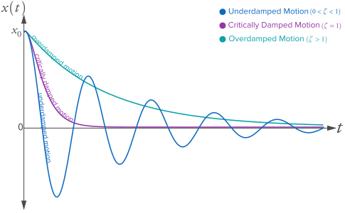
Although both the critically damped motion and the overdamped motion behave in a non-oscillatory fashion, there is a distinction between both. The overdamped case has a slower decaying rate than that of the critically damped case, illustrated in figure 5. Furthermore, as the damping ratio increases, the slower the transient response will be.
To wrap up, we've studied the response of the Mass Spring Damper System while no applied force is present. We've determined the mathematical model of the MSD system in three equivalent representations (eq.1, eq.2 and eq.3). Then, the mathematical model of the system was studied; we emphasized the difference between the three different cases of motion, namely the underdamped motion, the critically damped motion and the overdamped motion.
4) Simulation
In this section, you can try out different values of mass, spring coefficient, damper coefficient, damping ratio, and natural frequency. The position response will be depicted for the given values so that you get a feeling of the influence of the m, d, k, $\zeta$ and $\omega_n$ on the dynamical behavior of the system.